Working with the TAPE TimeSeries object

By contrast to the Ensemble, which operates on many lightcurves, the TAPE TimeSeries object operates on a single lightcurve.

Note: This notebook is limited as TimeSeries has a very initial implementation

From the Ensemble

A common use case for the Timeseries is pulling in an object of interest from the Ensemble. The Ensemble has a convenient exporter function for this purpose.

from tape import Ensemble, TimeSeries

ens = Ensemble()  # initialize an ensemble object

# Read in data from a parquet file
ens.from_parquet(
    "../../tests/tape_tests/data/source/test_source.parquet",
    id_col="ps1_objid",
    time_col="midPointTai",
    flux_col="psFlux",
    err_col="psFluxErr",
    band_col="filterName",
    sorted=True,
)

<tape.ensemble.Ensemble at 0x7ffad340dc30>

ts = ens.to_timeseries(88472935274829959)  # provided a target object id
ts.data

		midPointTai	psFlux	psFluxErr	filterName
band	index
r	0	58246.460938	18.149910	0.026191	r
	1	58249.441406	18.269829	0.028149	r
	2	58256.421875	18.243782	0.027706	r
	3	58259.445312	18.198299	0.026956	r
	4	58262.378906	18.211143	0.027165	r
...	...	...	...	...	...
g	93	59378.359375	18.968945	0.061589	g
	94	59382.382812	18.971306	0.061686	g
	95	59386.339844	18.872196	0.057729	g
	96	59392.300781	18.671389	0.050575	g
	97	59395.386719	19.070024	0.065927	g

499 rows × 4 columns

As a result, we get a multi-indexed Pandas DataFrame with data from a single lightcurve. The multi-index contains a band index as well as a integer index. We can operate on this as we normally would a Pandas DataFrame.

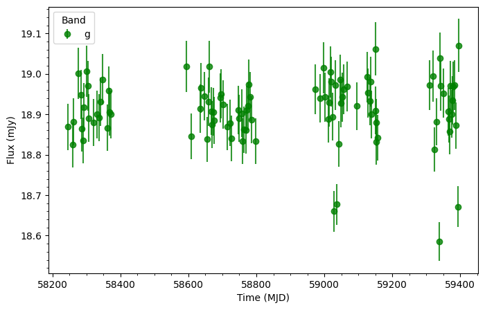
Below we plot out the g-band of the lightcurve.

import matplotlib.pyplot as plt


ts_g = ts.data[ts.band == "g"]

plt.figure(figsize=(8, 5))
plt.errorbar(ts_g.midPointTai, ts_g.psFlux, ts_g.psFluxErr, fmt="o", color="green", alpha=0.8, label="g")
plt.xlabel("Time (MJD)")
plt.ylabel("Flux (mJy)")
plt.minorticks_on()
plt.legend(title="Band", loc="upper left")

<matplotlib.legend.Legend at 0x7ffa97ee0ee0>