Explore SDSS Stripe 82 RR Lyrae catalog with period-folding

This short example notebook demonstrates how to use TAPE to explore the SDSS Stripe 82 RR Lyrae catalog. We will use a Lomb–Scargle periodogram to extract periods from r-band light curves and select the RR Lyrae star with the most confident period determination. Then, we will plot the period-folded light curve for this RR Lyrae star.

import matplotlib.pyplot as plt
from light_curve import Periodogram
from tape import Ensemble

# Load SDSS Stripe 82 RR Lyrae catalog
ens = Ensemble(client=False).from_dataset("s82_rrlyrae", sorted=True)

%%time

# Filter out invalid detections, "flux" denotes magnitude column
ens = ens.query("10 < flux < 25", table="source")

# Find periods using Lomb-Scargle periodogram
periodogram = Periodogram(peaks=1, nyquist=0.1, max_freq_factor=10, fast=False)

# Use r band only
df = ens.batch(periodogram, band_to_calc="r").compute()
display(df)

# Find RR Lyr with the most confient period
id = df.index[df["period_s_to_n_0"].argmax()]
period = df["period_0"].loc[id]

Using generated label, result_1, for a batch result.

	period_0	period_s_to_n_0
#id
4099	0.641751	19.061786
13350	0.547983	18.542068
15927	0.612275	17.760715
20406	0.631858	18.430296
21992	0.625867	20.105611
...	...	...
4956681	0.499531	14.800598
4983075	0.646707	21.350409
4984662	0.636876	19.130252
4992418	0.580378	20.278448
5011634	0.557231	19.749291

483 rows × 2 columns

CPU times: user 17.1 s, sys: 92.8 ms, total: 17.2 s
Wall time: 17.1 s

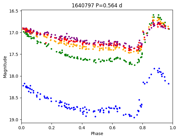
# Plot folded light curve
ts = ens.to_timeseries(id)
COLORS = {"u": "blue", "g": "green", "r": "orange", "i": "red", "z": "purple"}
color = [COLORS[band] for band in ts.band]
plt.title(f"{id} P={period:.3f} d")
plt.gca().invert_yaxis()
plt.scatter(ts.time % period / period, ts.flux, c=color, s=7)
plt.xlim([0, 1])
plt.xlabel("Phase")
plt.ylabel("Magnitude")

Text(0, 0.5, 'Magnitude')