Quickstart

The latest release of TAPE is installable via pip, using the following command:

%pip install lf-tape --quiet

Note: you may need to restart the kernel to use updated packages.

For more detailed installation instructions, see the Installation Guide.

TAPE provides a scalable framework for analyzing astronomical time series data. Let’s walk through a brief example where we calculate the Structure Function for a set of spectroscopically confirmed QSOs. First, we grab the available TAPE Stripe 82 QSO dataset:

from tape import Ensemble

ens = Ensemble()  # Initialize a TAPE Ensemble
ens.from_dataset("s82_qso", sorted=True)

<tape.ensemble.Ensemble at 0x7fe8c82f1ff0>

This dataset contains 9,258 QSOs, we can view the first 5 entries in the “object” table to get a sense of the available object-level information:

ens.head("object", 5)

	ra	dec	SDR5ID	M_i	M_i_corr	redshift	mass_BH	Lbol	u	g	r	i	z	Au
dbID
70	2.169302	1.238649	301	-23.901	-24.181	1.0730	0.000	0.000	20.793	20.469	20.197	20.040	20.000	0.116
98	1.091028	0.962126	144	-23.399	-23.576	0.7867	0.000	0.000	20.790	20.183	19.849	19.818	19.430	0.183
233	0.331289	0.177230	58	-24.735	-25.058	1.6199	0.000	0.000	20.892	20.554	20.431	20.199	20.099	0.154
1018	1.364696	-0.098956	190	-23.121	-24.045	0.6125	0.000	45.433	20.098	19.722	19.784	19.485	19.541	0.178
1310	0.221552	-0.292485	36	-26.451	-26.974	2.7563	9.361	46.760	20.707	19.663	19.610	19.705	19.529	0.174

The Ensemble stores data in two dask dataframes, object-level information in the “object” table as shown above, and individual time series measurements in the “source” table. As a result, many operations on the Ensemble closely follow operations on dask (and by extension pandas) dataframes. Let’s filter down our large QSO set to a smaller set with the total number of observations per object within a certain range:

ens.calc_nobs()  # calculates number of observations, produces "nobs_total" column
ens = ens.query("nobs_total >= 95 & nobs_total <= 105", "object")

We can now view the entirety of our remaining QSO set:

ens.compute("object")

	ra	dec	SDR5ID	M_i	M_i_corr	redshift	mass_BH	Lbol	u	g	r	i	z	Au	nobs_total
dbID
102187	2.815377	1.249789	406	-22.891	-23.368	0.5804	8.023	45.571	20.777	20.368	19.950	19.570	19.273	0.142	95
138158	10.133773	-0.230790	1541	-22.266	-22.827	0.2419	8.332	45.131	19.090	18.857	18.485	18.085	18.033	0.117	105
187596	10.556096	0.988253	1615	-22.652	-23.392	0.3289	8.392	45.321	19.915	19.185	18.589	18.423	17.770	0.105	95
711662	15.176414	1.083781	2359	-22.703	-23.310	0.6383	0.000	0.000	20.942	20.491	20.330	19.979	19.815	0.117	100
762267	343.360626	0.507056	75223	-22.187	-23.001	0.4627	7.856	45.186	21.107	20.647	20.193	19.855	19.529	0.465	95
1128581	339.200653	1.190031	74754	-24.092	-24.483	0.5481	0.000	45.471	20.410	19.395	18.889	18.333	18.346	0.398	95
1250783	28.063360	0.648427	4283	-23.270	-24.417	0.8656	8.432	45.550	20.865	20.368	20.131	20.169	19.936	0.158	105
1254675	29.243357	0.271094	4485	-22.436	-23.097	0.3593	7.834	45.277	19.277	19.202	19.007	18.873	18.387	0.161	105
1266724	26.613321	0.350273	4077	-22.295	-22.739	0.4051	8.177	45.200	19.993	19.623	19.428	19.300	18.959	0.154	105
1393824	333.115570	0.861277	73967	-26.207	-26.783	1.7729	9.260	46.675	19.617	19.396	19.341	18.971	18.955	0.235	105
1664567	34.941772	-0.079720	5397	-22.491	-23.066	0.5550	8.111	45.226	20.446	20.109	20.209	19.878	19.660	0.185	95
1988699	36.283642	0.285343	5594	-23.966	-24.449	0.5269	8.872	45.810	18.807	18.357	18.501	18.290	18.265	0.217	105
3776342	53.202126	-0.365366	8031	-25.769	-26.098	1.7134	9.438	46.518	20.075	19.873	19.751	19.475	19.374	0.594	105
3777871	51.230343	0.040977	7747	-22.299	-22.636	0.4801	8.185	45.105	20.592	20.272	20.220	19.896	19.482	0.622	105
3800671	54.261101	1.107667	-1	-22.000	-1.000	0.4280	-1.000	-1.000	20.540	20.300	19.950	19.410	18.870	0.000	100
3867529	54.385761	0.929904	8183	-22.200	-23.229	0.6244	0.000	0.000	21.516	21.335	21.118	20.557	20.189	0.436	100
3954424	358.399628	-1.110925	77189	-24.394	-23.636	1.2966	8.743	46.149	20.346	20.331	20.129	20.011	19.905	0.144	105
4938823	55.578239	0.702042	8370	-22.515	-22.261	0.5520	0.000	0.000	20.938	20.591	20.427	20.034	19.599	0.661	105
4970580	57.908497	0.332248	8579	-22.204	-22.744	0.3815	8.646	45.254	21.351	20.761	20.143	19.658	18.865	1.169	95
4974467	55.593185	-0.571577	-1	-24.400	-1.000	2.3700	-1.000	-1.000	20.580	20.840	20.370	20.470	20.590	0.000	100

Finally, we can calculate the Structure Function for each of these QSOs, using the available TAPE Structure Function Module:

from tape.analysis import calc_sf2

result = ens.batch(
    calc_sf2, sf_method="macleod_2012"
)  # The batch function applies the provided function to all individual lightcurves within the Ensemble
result.compute()

Using generated label, result_1, for a batch result.

		lc_id	band	dt	sf2	1_sigma
dbID
102187	0	102187	g	212.944457	7906.087066	0.0
	1	102187	g	1113.928944	0.058018	0.0
	2	102187	i	212.944457	0.016962	0.0
	3	102187	i	1113.928944	0.017595	0.0
	4	102187	r	212.944457	0.008150	0.0
...	...	...	...	...	...	...
4974467	5	4974467	r	1857.713042	0.041112	0.0
	6	4974467	u	330.626307	1.099520	0.0
	7	4974467	u	1857.713042	3233.746505	0.0
	8	4974467	z	330.626307	1.714607	0.0
	9	4974467	z	1857.713042	2.537171	0.0

250 rows × 5 columns

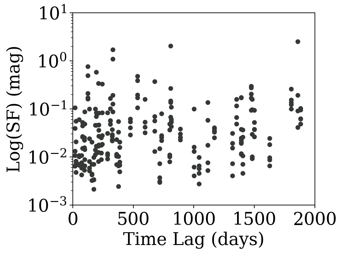
The result is a table of delta times (dts) and structure function (sf2) for each unique lightcurve (labeled by lc_id). We can now visualize our delta times versus the computed structure function for each unique object.

import matplotlib.pyplot as plt
from matplotlib import rcParams

%matplotlib inline
%config InlineBackend.figure_format = "retina"
rcParams["savefig.dpi"] = 550
rcParams["font.size"] = 20
plt.rc("font", family="serif")

fig, ax = plt.subplots(nrows=1, ncols=1, figsize=(5, 4))
plt.scatter(result["dt"], result["sf2"], s=20, alpha=1, color="#353935")
plt.yscale("log")
plt.ylabel("Log(SF) (mag)")
plt.xlabel("Time Lag (days)")
plt.ylim(1e-3, 1e1)
plt.xlim(0, 2e3)

(0.0, 2000.0)

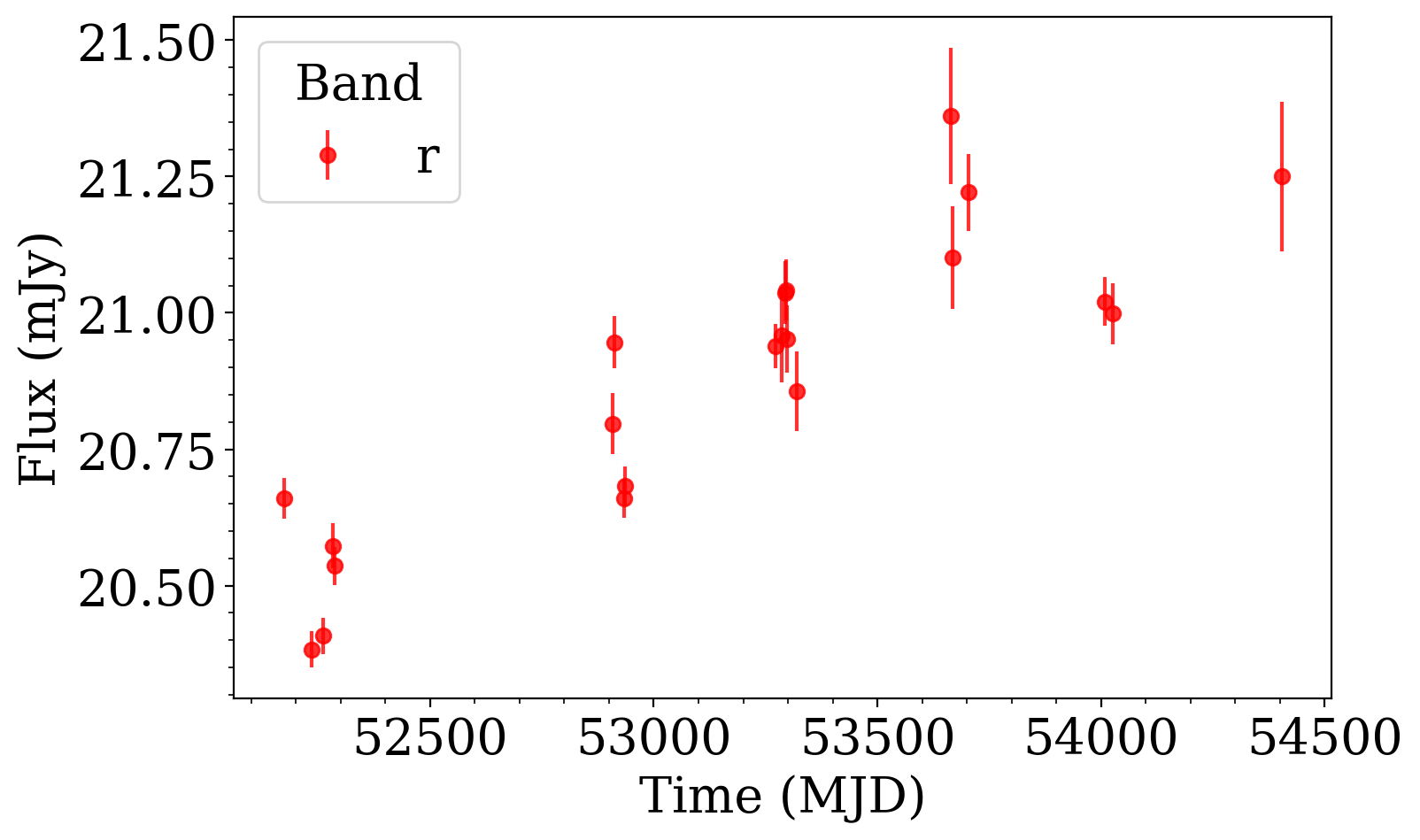
Finally, suppose we want to select the ID with the maximum sf2 value from the computed feature. Using the available ens.to_timeseries() that creates a TimeSeries object, we can access the light curve for the target ID.

max_id = result.compute()["sf2"].idxmax()[0]
lc = ens.to_timeseries(max_id)
lc

<tape.timeseries.TimeSeries at 0x7fe8b26405b0>

filter_r = lc.band == "r"  # select filter

plt.figure(figsize=(8, 5))
plt.errorbar(
    lc.time[filter_r], lc.flux[filter_r], lc.flux_err[filter_r], fmt="o", color="red", alpha=0.8, label="r"
)
plt.minorticks_on()
plt.ylabel("Flux (mJy)")
plt.xlabel("Time (MJD)")
plt.legend(title="Band", loc="upper left")

<matplotlib.legend.Legend at 0x7fe876bf5960>